PG_Project 2: Identify Deepfakes with GAN
Introduction
The rise of synthetic media created using powerful techniques from Machine Learning (ML) and Artificial Intelligence (AI), has garnered attention across multiple industries in recent years. Deepfakes, as they are aptly named, have been used to misrepresent well-known politicians in videos, impersonate female celebrities in pornography, and in social engineering schemes, enabling identity theft and other fraudulent behavoir.
ypically, deepfakes are made using a neural network-based architecture, the most capable of which utilizes generative adversarial networks (GANs). This involves placing two neural networks in contest with one another: the first generates new data from the same statistical distribution as the training set, and the second attempts to discriminate data produced by the first from data in the original training set. Contesting the two tends to improve both the quality of the ‘fake’ data produced by the first network as well as the discrimination ability of the second. Naturally, this implies that the best way to combat deepfakes is to use the same techniques that produce them: GANs.
This project aims to demonstrate the approach and improve on the GAN settings so that can produce a better solution.
Basic Structure Of A GAN
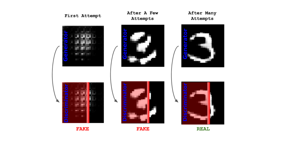
As I mentioned before, the core concept of GANs lies in pitting two neural networks against each other in an opposing fashion. The concept was first elucidated by Goodfellow et al. in their 2014 paper. In this article, we’ll use one of the datasets from their paper: the MNIST dataset of greyscale handwritten digits. Image datasets are typically computationally heavy, but I was able to run the models on these images with modest hardware and in a reasonable amount of time. In our case, the Generator Neural Network (GNN) will attempt to create images that look like they could come from the original dataset. On the other hand, the Discriminator Neural Network (DNN) will try to distinguish between images that are produced by the generator and the images from the original dataset.
In theory, the generator will become increasingly better at creating images that resemble the original images throughout the training. On the other hand, the discriminator converges to a state where it cannot differentiate between the fake dataset and the original (or rather, the probability that it is a fake approaches 50%). This process is illustrated below:
How To Implement A GAN With TensorFlow
To implement this in Python, we first import the dataset. Each image is 28 x 28 pixels, with a grayscale value assigned to each pixel. The greyscale values range from 0 (white) to 255 (black). It is best practice to normalize these values to obtain optimal behavior (especially with values around 0). I’m choosing to normalize values from -1 (white) to 1 (black). The images have already been centered and cropped. Finally, we’ll randomly sample the images and divide the set into batches of 256.
train_images, train_labels), (_, _) = tf.keras.datasets.mnist.load_data()

train_images = train_images.reshape(train_images.shape[0], 28, 28, 1).astype('float32')
train_images = (train_images - 127.5) / 127.5
BUFFER_SIZE = 60000
BATCH_SIZE = 256
train_dataset = tf.data.Dataset.from_tensor_slices(train_images).shuffle(BUFFER_SIZE).batch(BATCH_SIZE)
To create the generator, we’ll use a feedforward neural network. The input to the network is random noise, and at the end of the network we want to end up with an output shape matching the dimensions of the original images. We’ll start with a regular, densely connected layer with 7 x 7 x 256 units, then use a series of upsampling layers (deconvolution) to reach the desired image size of 28 x 28 x 1. A combination of ReLU activation functions and hyperbolic tangents are used:
def make_generator_model():
    model = tf.keras.Sequential()
    model.add(layers.Dense(7*7*256, use_bias=False, input_shape=(100,)))
    model.add(layers.BatchNormalization())
    model.add(layers.LeakyReLU())

    model.add(layers.Reshape((7, 7, 256)))
    assert model.output_shape == (None, 7, 7, 256) # Note: None is the batch size

    model.add(layers.Conv2DTranspose(128, (5, 5), strides=(1, 1), padding='same', use_bias=False))
    assert model.output_shape == (None, 7, 7, 128)
    model.add(layers.BatchNormalization())
    model.add(layers.LeakyReLU())

    model.add(layers.Conv2DTranspose(64, (5, 5), strides=(2, 2), padding='same', use_bias=False))
    assert model.output_shape == (None, 14, 14, 64)
    model.add(layers.BatchNormalization())
    model.add(layers.LeakyReLU())

    model.add(layers.Conv2DTranspose(1, (5, 5), strides=(2, 2), padding='same', use_bias=False, activation='tanh'))
    assert model.output_shape == (None, 28, 28, 1)

    return model
To test the function, we can generate a fake image (without training the net) with a single noise seed input:
generator = make_generator_model()

noise = tf.random.normal([1, 100])
generated_image = generator(noise, training=False)
To plot the image produced:
Data distribution for the binary outcome variable,
plt.figure(figsize=(12,12))
plt.imshow(generated_image[0, :, :, 0], cmap='gray')
plt.show()
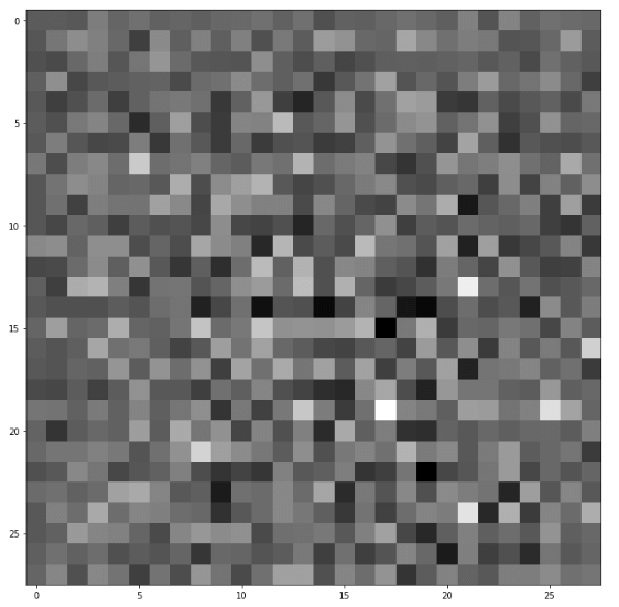
The net successfully creates an image matching the 28 x 28 pixel size with sufficient randomness. To see a summary of the layers of the net:
generator.summary()
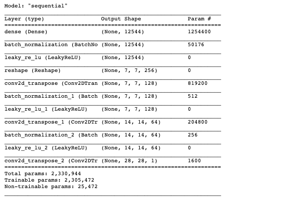
Now we can do something similar to make the discriminator network:
def make_discriminator_model():
    model = tf.keras.Sequential()
    model.add(layers.Conv2D(64, (5, 5), strides=(2, 2), padding='same',
                                    input_shape=[28, 28, 1]))
    model.add(layers.LeakyReLU())
    model.add(layers.Dropout(0.3))

    model.add(layers.Conv2D(128, (5, 5), strides=(2, 2), padding='same'))
    model.add(layers.LeakyReLU())
    model.add(layers.Dropout(0.3))

    model.add(layers.Flatten())
    model.add(layers.Dense(1))

    return model
In this case, we want the input dimensions to match a single image dimension, and the output to be a single number quantifying the degree to which the image is fake or real. To test the net, we can use the previously generated fake image:
discriminator = make_discriminator_model()
decision = discriminator(generated_image)
print(decision)
Output:
tf.Tensor([[0.00022886]], shape=(1,1), dtype=float32)
Of course, the model is not trained yet, but the idea is to output positive values for real images and negative values for fake images. This is implemented when we define the losses for each network. To see a summary of the discriminator network:
discriminator.summary()
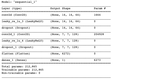
Now that we have both the networks in place, we need to define loss functions for each. As mentioned previously, we want the discriminator to output more positive numbers for real images and more negative numbers for fake images. To implement this, we compare the discriminator’s predictions on real images to an array of 1s, and the discriminator’s predictions on fake images to an array of 0s.
cross_entropy = tf.keras.losses.BinaryCrossentropy(from_logits=True)

def discriminator_loss(real_output, fake_output):
    real_loss = cross_entropy(tf.ones_like(real_output), real_output)
    fake_loss = cross_entropy(tf.zeros_like(fake_output), fake_output)
    total_loss = real_loss + fake_loss
    return total_loss

def generator_loss(fake_output):
    return cross_entropy(tf.ones_like(fake_output), fake_output)

generator_optimizer = tf.keras.optimizers.Adam(1e-4)
discriminator_optimizer = tf.keras.optimizers.Adam(1e-4)
When running models on datasets this large, it is a good idea to implement checkpoint saves during the training loops:
checkpoint_dir = './training_checkpoints'
checkpoint_prefix = os.path.join(checkpoint_dir, "ckpt")
checkpoint = tf.train.Checkpoint(generator_optimizer=generator_optimizer,
                          discriminator_optimizer=discriminator_optimizer,
                          generator=generator,
                          discriminator=discriminator)
From here, we have all the tools needed to establish the training procedure for the networks. To do so, we’ll define a single function for each training step, along with a training function that loops over the train step function, saves the images produced by the generator network, as well as any checkpoints. At each training step, a random seed is used to generate images. The discriminator is then used to classify real images and fakes images. We then calculate the loss of each of the models, and update the weights in each network using the gradients.
@tf.function
def train_step(images):
    noise = tf.random.normal([BATCH_SIZE, noise_dim])

    with tf.GradientTape() as gen_tape, tf.GradientTape() as disc_tape:
        generated_images = generator(noise, training=True)

        real_output = discriminator(images, training=True)
        fake_output = discriminator(generated_images, training=True)

        gen_loss = generator_loss(fake_output)
        disc_loss = discriminator_loss(real_output, fake_output)

    gradients_of_generator = gen_tape.gradient(gen_loss, generator.trainable_variables)
    gradients_of_discriminator = disc_tape.gradient(disc_loss, discriminator.trainable_variables)

    generator_optimizer.apply_gradients(zip(gradients_of_generator, generator.trainable_variables))
    discriminator_optimizer.apply_gradients(zip(gradients_of_discriminator, discriminator.trainable_variables))
The following function generates and saves the images:
def generate_and_save_images(model, epoch, test_input):
    predictions = model(test_input, training=False)
    fig = plt.figure(figsize=(4,4))
    for i in range(predictions.shape[0]):
        plt.subplot(4, 4, i+1)
        plt.imshow(predictions[i, :, :, 0] * 127.5 + 127.5, cmap='gray')
        plt.axis('off')
    plt.savefig('image_at_epoch_{:04d}.png'.format(epoch))
    plt.show()
Finally, we’ll define the train function:
def train(dataset, epochs):
    for epoch in range(epochs):
        start = time.time()
        for image_batch in dataset:
            train_step(image_batch)
        display.clear_output(wait=True)
        generate_and_save_images(generator,epoch + 1,seed)
        if (epoch + 1) % 5 == 0:
            checkpoint.save(file_prefix = checkpoint_prefix)
            print('Time for epoch {} is {} sec'.format(epoch + 1, time.time()-start))
    display.clear_output(wait=True)
    generate_and_save_images(generator,epochs,seed)
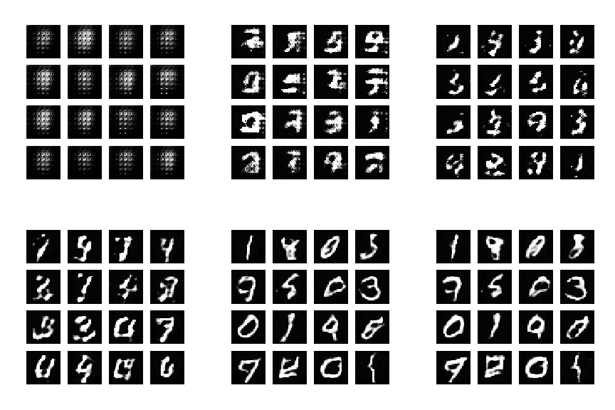
Now we can actually train the model. I recommend doing around 50 epochs to converge on realistic fake images. With the modest hardware that I am using (1.6 GHz Intel Core i5), each epoch takes approximately 10 minutes. In this case, I ran the model overnight to obtain the images in the gif below.
EPOCHS = 50
noise_dim = 100
num_examples_to_generate = 16

seed = tf.random.normal([num_examples_to_generate, noise_dim])

train(train_dataset, EPOCHS)
The training will populate the current directory with an image for each epoch. We can use the imageio and glob packages to create a gif showing the progression of the generator images:
import imageio
import glob

anim_file = 'dcgan.gif'

with imageio.get_writer(anim_file, mode='I') as writer:
    filenames = glob.glob('image*.png')
    filenames = sorted(filenames)
    last = -1
    for i,filename in enumerate(filenames):
        frame = 2*(i**0.5)
        if round(frame) > round(last):
            last = frame
        else:
            continue
        image = imageio.imread(filename)
        writer.append_data(image)
    image = imageio.imread(filename)
    writer.append_data(image)
When finished, you should get something like this:
Conclusion
The Best Way To Combat Deepfakes Is To Use The Same Technique That Produces Them: GAN.
References
- Sample code on my github repo.
- TensorFlow Optimization Showdown: ActiveState vs. Anaconda
- Deploying a Dog Identification TensorFlow Model Using Python and Flask
Last updated: 24/03/2020


