Linear Regression in Python
What is Linear Regression (LR)?
- Linear regression (LR) models the relationship between the explanatory/independent/predictor/regressor/exogeneous (X) variable with that of dependent/response/criterion/endogeneous variable (Y)
- For example, how the likelihood of blood pressure is influenced by a person’s age and weight. This relationship can be explained using linear regression
- In LR, the Y variable should be continuous whereas the X variable can be continuous or categorical. If both X and Y are continuous, the linear relationship can be estimated using correlation coefficient (r) or the coefficient of determination (r-squared)
- LR is useful if the relationships between the X and Y variables are linear
- LR is helpful to predict the value of Y based on the value of the X variable
Types of Linear Regression (LR)?
- Univariate LR: Linear relationships between Y and X variables can be explained by single X variable
\( Y = a + bX + \epsilon \)
Where, a = y-intercept, b = slope of the regression line and \( \epsilon \) = error term (residuals)
-
Multiple LR: Linear relationships between Y and X variables can be explained by multiple X variables
\( Y = a + b_1X_1 + b_2X_2 + b_3X_3 + ... + b_nX_n + \epsilon \)
Where, a = y-intercept, b = slope of the regression line and \( \epsilon \) = error term (residuals) - The y-intercept (a) is a constant and slope (b) of regression line is a regression coefficient.
- How to perform multiple linear regression?
Linear Regression (LR) Assumptions
- Relationship between the X and Y variables should be linear
- Errors (residuals) should be independent of each other
- Errors (residuals) should be normally distributed with mean of 0
- Errors (residuals) should have equal variance (Homoscedasticity)
Linear Regression (LR) Outputs
Correlation coefficient (r)
- r describes a linear relationship between X and Y variables
- r > 0 indicates a positive linear relationship between X and Y variables. As one of the variable increases, the other variable also increases. r = 1 is a perfect positive linear relationship
- Similarly, r < 0 indicates a negative linear relationship between X and Y variables. As one of the variable increases, the other variable decreases, and vice versa. r = -1 is perfect negative linear relationship
- r = 0 indicates, there is no linear relationship between the X and Y variables
Coefficient of determination (r-squared)
- r-squared is a square of correlation coefficient (r) and usually represented as percentages
- r-squared explains the variation in the Y variable that is explained by the fitted regression line
- r-squared can range from 0 to 1 (0 to 100%). r-squared = 1 (100%) indicates that the fitted regression line explains all the variability of Y variable around its mean.
Residuals (regression error)
- Residuals or error in regression represents the distance of the observed data points from the predicted regression line
\( residuals = predicted \ Y \ (\hat{y}_i) - actual \ Y (y_i) \)
Root Mean Square Error (RMSE)
- RMSE represents the standard deviation of the residuals. It gives an estimate of the spread of observed data points across the predicted regression line
Linear Regression (LR) in Python
- We will use
bioinfokit v0.7.1or later for performing LR. - Check How to install bioinfokit for latest version.
- Download dataset
Perform Linear Regression (LR)
# you can use interactive python interpreter, jupyter notebook, google colab, spyder or python code
# I am using interactive python interpreter (Python 3.8.2)
>>> from bioinfokit.analys import stat, get_data
# load dataset as pandas dataframe
# should not have missing values (NaN)
>>> df = get_data('slr').data
>>> df.head()
   X1    Y
0  25  670
1  30  690
2  18  635
3  15  625
4  20  640

# LR with one independent variable
>>> reg= stat()
>>> reg.lin_reg(df=df, x=["X1"], y=["Y"])

# output
Regression equation:

569.0916 + (3.7515*X1)

Regression Summary:


----------------------------------------  --------
Dependent variables                       ['X1']
Independent variables                     ['Y']
Coefficient of determination (r-squared)  0.918
Adjusted r-squared                        0.9141
Root Mean Square Error (RMSE)             6.6718
Mean of Y                                 639.3913
Residual standard error                   6.9808
No. of Observations                       23

Regression Coefficients:

Parameter      Estimate    Std Error    t-value    P-value Pr(>|t|)
-----------  ----------  -----------  ---------  ------------------
Intercept     569.092         4.8094   118.329           3.7802e-31
X1              3.75149       0.2446    15.3373          7.0019e-13


ANOVA Summary:

Source      Df    Sum Squares  Mean Squares    F         Pr(>F)
--------  ----  -------------  --------------  --------  ----------
Model        1       11462.1   11462.1214      235.2108  7.0080E-13
Error       21        1023.36  48.7313
Total       22       12485.5

# you can check predicted response (y_hat)
>>> reg.y_hat
Interpretation
- The regression line with equation [Y = 569.0916 + (3.7515*X1)], is helpful to predict the value of the Y variable from the given value of the X1 variable. In general, a regression can be useful in predicting the Y of any value within the range of X1. It can be also used to predict Y from X outside the given range, but such extrapolation may not be useful
- The slope (3.7515) represents the change in the Y per unit change in the X1 variable. It means that the value Y increases by 3.7515 with each unit increase in X1
- The intercept (569.0916) represents the value of Y at X1 = 0. Here need to be cautious to interpret intercept as sometimes the value (X1=0) does not make any sense (e.g. speed of car or height of the person). In such cases, the values within the range of X1 should be considered to interpret the intercept
- The coefficient of determination (r-squared) is 0.918 (91.8%), which suggests that 91.8% of the variance in Y can be explained by X1 alone. Adjusted r-squared is useful where there are multiple X variables in the model (multiple linear regression)
- The correlation coefficient (r) is 0.9581, which suggests that there is a positive relationship between X and Y variables. As X1 increases, Y also increases
- From Regression Coefficients, the P-value obtained for X1 independent variable is significant (<0.05), it suggests that X1 significantly influence the response variable Y (there is a significant relationship between X1 and Y)
- From ANOVA, the P-value is significant (<0.05), which suggests that there is a significant relationship between X1 and Y. The X1 variable can reliably predict the Y variable.
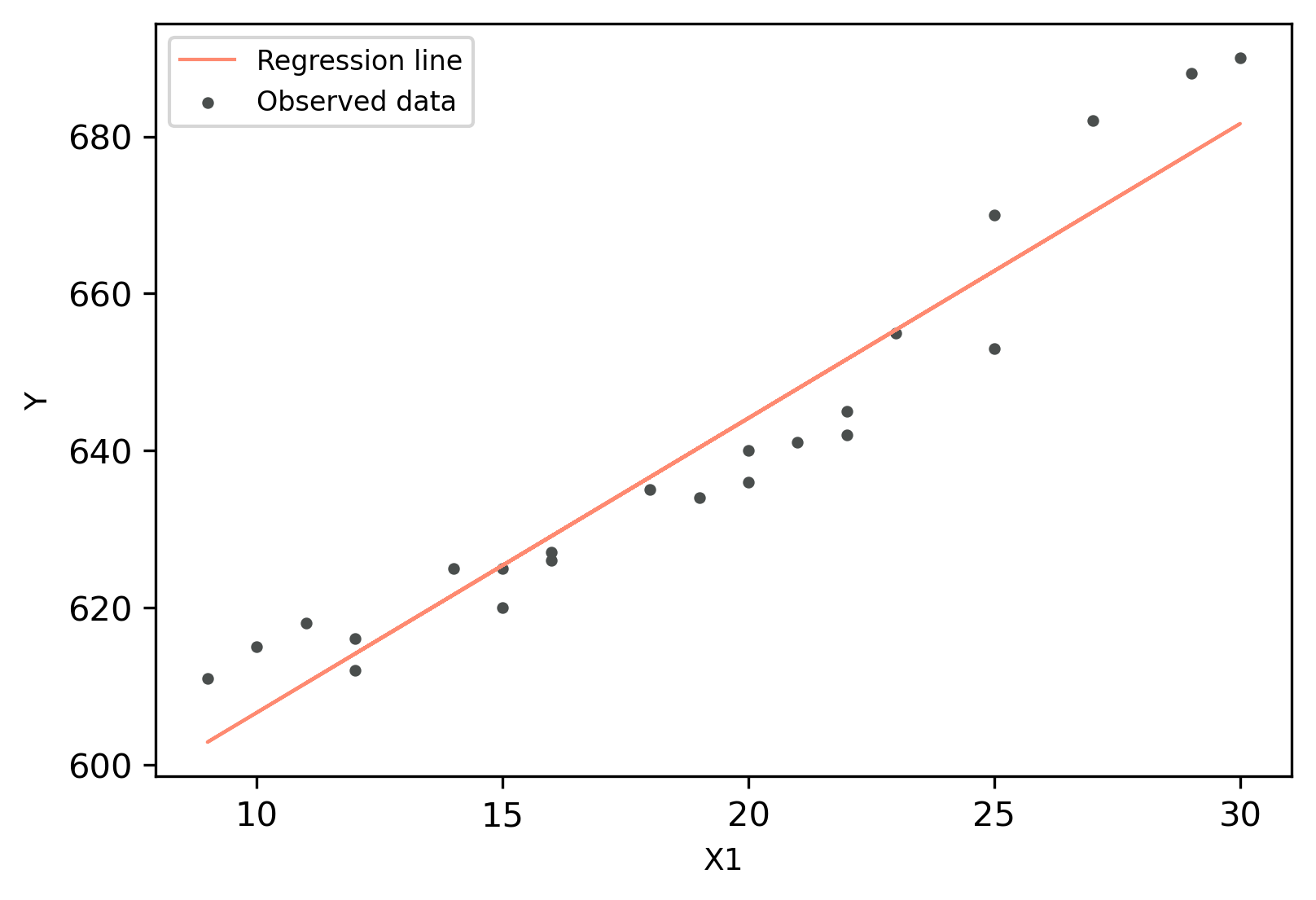
Linear Regression (LR) plot
Generate regression plot,
>>> import pandas as pd
>>> from bioinfokit import visuz
# get predicted Y and add to original dataframe
>>> df['yhat']=reg.y_hat
>>> df.head()
   X1    Y        yhat
0  25  670  662.878924
1  30  690  681.636398
2  18  635  636.618460
3  15  625  625.363976
4  20  640  644.121450

# create regression plot with defaults
>>> visuz.stat.regplot(df=df, x='X1', y='Y', yhat='yhat')
# plot will be saved in same dir (reg_plot.png)
# set parameter show=True, if you want view the image instead of saving
Check Linear Regression (LR) Assumptions
Residuals vs fitted (y_hat) plot: This plot used to check for linearity, variances and outliers in the regression data
# get residuals and standardized residuals and add to original dataframe
>>> df['res']=reg.residuals
>>> df['std_res']=reg.std_residuals
>>> df.head()
   X1    Y        yhat       res   std_res
0  25  670  662.878924  7.121076  1.017297
1  30  690  681.636398  8.363602  1.194800
2  18  635  636.618460 -1.618460 -0.231209
3  15  625  625.363976 -0.363976 -0.051997
4  20  640  644.121450 -4.121450 -0.588779

# create fitted (y_hat) vs residuals plot
>>> visuz.stat.reg_resid_plot(df=df, yhat='yhat', resid='res', stdresid='std_res')
# plot will be saved in same dir (resid_plot.png and std_resid_plot.png)
# set parameter show=True, if you want view the image instead of saving

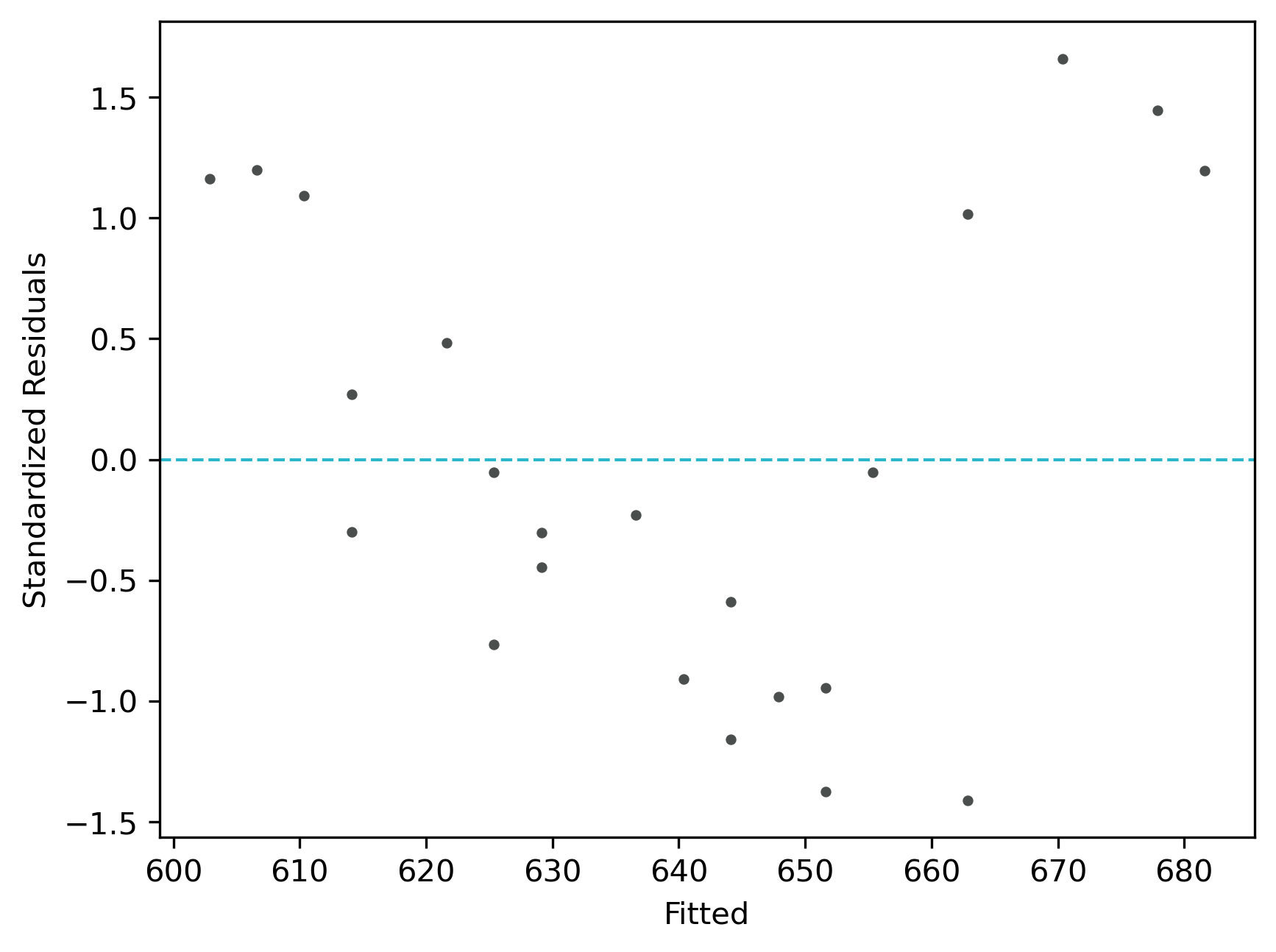
From the plot,
- As the data is pretty equally distributed around the line=0 in the residual plot, it meets the assumption of residual equal variances. The outliers could be detected here if the data lies far away from the line=0.
- In the standardized residual plot, the residuals are within -2 and +2 range and suggest that it meets assumptions of linearity
Quantile-quantile (QQ) plot: This plot used to check the data normality assumption
# you can use interactive python interpreter, jupyter notebook, spyder or python code
# I am using interactive python interpreter (Python 3.7)
>>> import statsmodels.api as sm
>>> import matplotlib.pyplot as plt
# check dataframe for required variables (we will need std_res variable for QQ plot)
>>> df.head()
   X1    Y        yhat       res   std_res
0  25  670  662.878924  7.121076  1.017297
1  30  690  681.636398  8.363602  1.194800
2  18  635  636.618460 -1.618460 -0.231209
3  15  625  625.363976 -0.363976 -0.051997
4  20  640  644.121450 -4.121450 -0.588779

# create QQ plot
# line=45 option to plot the data around 45 degree line
>>> sm.qqplot(df['std_res'], line='45')
>>> plt.xlabel("Theoretical Quantiles")
>>> plt.ylabel("Standardized Residuals")
>>> plt.show()
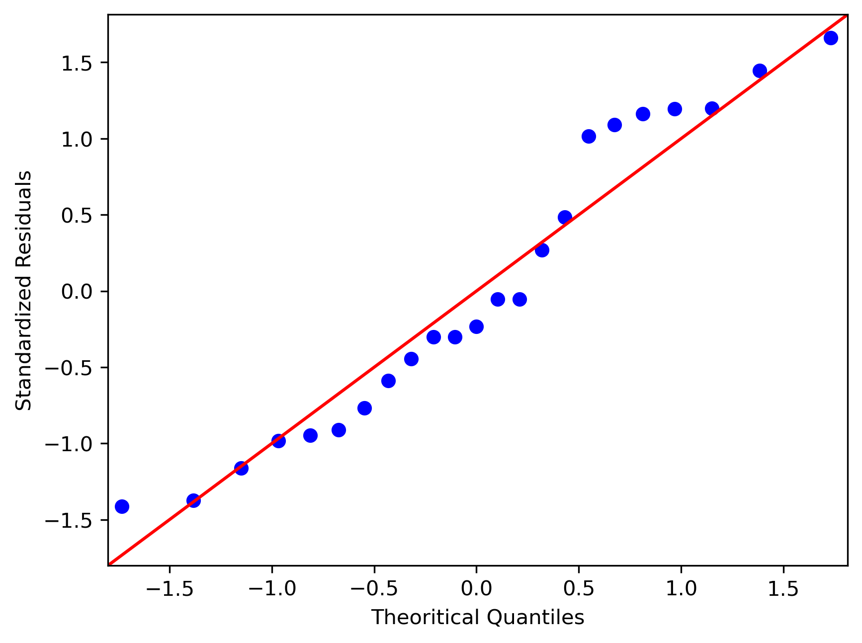
From the plot,
- As the standardized residuals lie around the 45-degree line, it suggests that the residuals are normally distributed
Check for How to perform multiple linear regression?
Linear Regression with PyTorch
Let’s perform a LR with PyTorch with the same dataset
>>> from bioinfokit.analys import stat, get_data
>>> import torch as th
>>> df = get_data('slr').data
>>> df.head()
   X1    Y
0  25  670
1  30  690
2  18  635
3  15  625
4  20  640

# convert to PyTorch tensor
# variable shape should be (samples, features)
>>> X1 = th.tensor(df[['X1']].values, dtype=th.float32)
>>> Y = th.tensor(df[['Y']].values, dtype=th.float32)

# LR model using PyTorch
>>> in_features = 1 # number of independent variable
>>> out_features = 1 # dim of predicted variable
>>> lr_model = th.nn.Linear(in_features, out_features)

# define loss function (regression error)
>>> mse_loss = th.nn.MSELoss()
# optimize to minimize the loss function and find optimal LR parameters (Regression Coefficients)
>>> optimizer = th.optim.SGD(lr_model.parameters(), lr=0.002)
# set number of iterations until you see the convergence in the loss function
# when you see similar minimum values for a large number of ending iterations
# it will give you the best values of LR parameters
>>> n_iter = 20000
>>> for i in range(n_iter):
        # predict model with current LR parameters
        y_pred = lr_model(X1)
        # calculate loss function
        step_loss = mse_loss(y_pred, Y)

        # Backward to find the derivatives of the loss function with respect to LR parameters
        # make any stored gradients to zero
        optimizer.zero_grad()
        step_loss.backward()
        # update with current step LR parameters
        optimizer.step()

        print ('i [{}], Loss: {:.2f}'.format(i, step_loss.item()))

# see the last few iterations
i [19986], Loss: 44.51
i [19987], Loss: 44.51
i [19988], Loss: 44.51
i [19989], Loss: 44.51
i [19990], Loss: 44.51
i [19991], Loss: 44.51
i [19992], Loss: 44.51
i [19993], Loss: 44.51
i [19994], Loss: 44.51
i [19995], Loss: 44.51
i [19996], Loss: 44.51
i [19997], Loss: 44.51
i [19998], Loss: 44.51
i [19999], Loss: 44.51
Now, get the best LR parameters from this trained model,
# intercept (a)
>>> lr_model.bias.item()
568.7089233398438
# slope (b)
>>> lr_model.weight.item()
3.7700467109680176
Generate regression plot,
>>> from bioinfokit.visuz import stat
# detach will not build a gradient computational graph (no backpropagation)
>>> y_pred = lr_model(X1).detach()
>>> df['yhat']=y_pred.numpy()
>>> stat.regplot(df=df, x='X1', y='Y', yhat='yhat')

Now, let’s predict the Y from some random X1,
>>> X1_data = 28
# predict Y value when X1 is 28
>>> y_pred = lr_model(th.tensor([[X1_data]], dtype=th.float32)).detach()
>>> y_pred.item()
674.2701416015625
# Y=674.27 when X1 is 28
Last updated: July 12, 2020