UG Research project: Predictive Modeling Of Air Quality

Introduction

In many parts of the world, air quality is compromised by the burning of fossil fuels, which release particulate matter small enough to penetrate the lungs. This kind of air pollution has been linked to increases in respiratory, cardiovascular and cancer mortality.

As computational power and the sheer amount of available data increases, the viability of predictive models (ie., machine learning-based models that provide a statistical likelihood of an outcome) are gaining ground as an alternative solution to many contemporary problems. Air quality is one of the most concern problem. Using existing data we should be able to predict the sir quality in the near future. Python is a powerful tool for predictive modeling, and is relatively easy to learn. This project is exactly doing that.

Modeling Weather vs Particulate Matter Concentration

The dataset we will be using is from the UCI Machine Learning Repository and contains two different sets of information:

• Hourly meteorological data from the Beijing Capital International Airport.
• PM2.5 data from the US Embassy in Beijing.
• PM2.5 refers to atmospheric Particulate Matter (PM) that is less than 2.5 micrometers in diameter It is reasonable to expect that the concentration of PM2.5 would be affected by the local weather. Understanding the relationship (i.e. building a predictive model) between PM2.5 and weather could provide actionable intelligence without the need to invest in additional PM2.5 monitoring stations, which is a much more expensive solution.

Note that the Beijing Capital International Airport is located about 20km from the US Embassy, so we will assume the weather data is more or less uniform across the city for the sake of this analysis.

Importing & Cleaning Data with Pandas

Before a prediction model can be built you need to do data preprocessing. It generally involves data cleaning, transformation and formalization etc. The degree to which cleaning is necessary depends on the source, but more often than not, it is the first hurdle for any data scientist. Fortunately, the pandas package provides the tools to do so. you may need to do something similar to this:

import pandas as pd

data_df = pd.DataFrame(pd.read_csv('PRSA_data_2010.1.1-2014.12.31.csv', index_col = 0))
data_df.head()

If you are Lucky, like this data, it is in relatively good shape. The output should look like this:

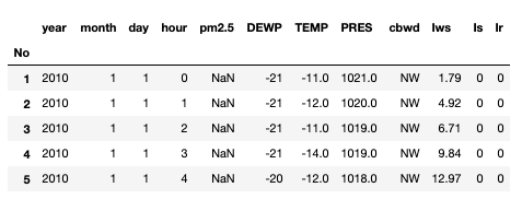
The first thing to note is that four of the features are all time indicators for each observation. These can easily be coerced into a single feature:

data_df['datetime'] = pd.to_datetime(data_df[['year', 'month','day', 'hour']])
data_df = data_df.drop(['year', 'month','day', 'hour'], axis = 1)

It is also clear that there are Not a Number (NaN) values in the PM2.5 column:

data_df.isnull().sum()

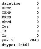
This is a bit inconvenient, as it is the variable that we hope to predict. To resolve this there are several options:

• Drop the rows with missing values altogether
• Impute the values in reference to other values in the same column
• Impute the values using the other features in each row

data_df = data_df[['datetime', 'DEWP', 'TEMP', 'PRES', 'cbwd', 'Iws', 'Is', 'Ir', 'pm2.5']].iloc[24:].reset_index().drop('No', axis = 1)
data_df[['pm2.5']] = data_df[['pm2.5']].interpolate(method='linear')

I am also choosing to make the following adjustments to the data:

• Drop the first 24 observations, as they don’t have a previous value to interpolate with.
• Drop the unnecessary No column, as the pandas index serves the same function

Now we have some clean data to work with:

data_df.head()

Creating A Simple Predictive Model

Our goal is to build a model to predict the PM2.5 concentration in a given hour based on the weather factors in the dataset: dew point, temperature, pressure, combined wind direction, wind speed, cumulated hours of snow, and cumulated hours of rain. The simplest approach is to use these features as-is, without any modification. Since most of the data is numerical, the simplest statistical model to apply is an ordinary Least Squares Regression model. To do so, we first break up the dataset into a test and training set. We will build the model with the training set, and evaluate its performance with the test set. This ensures the model is as unbiased as possible. To do so:

from sklearn.model_selection import train_test_split

data_df = data_df.set_index('datetime')
X_train, X_test, y_train, y_test = train_test_split(data_df[['DEWP', 'TEMP', 'PRES', 'Iws', 'Is', 'Ir']], data_df[['pm2.5']], test_size=0.2)

And to construct the model, we can use the statsmodel package:

import statsmodels.api as sm
import numpy as np

model = sm.OLS(np.asarray(y_train), np.asarray(X_train))
results = model.fit()
print(results.summary())

The output produces a summary of the regression results and fit parameters for each of the features:

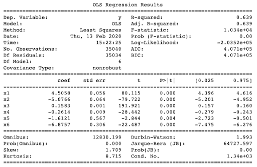
The R-squared value is extremely poor at just 0.639. To obtain a better understanding of how the model performs, we can run the test set through a Root Mean Square Error (RSME) calculation. This tells us how far the predictions are from the actual values, on average.

from sklearn.metrics import mean_squared_error

y_pred = results.predict(np.asarray(X_test))
mse = mean_squared_error(np.asarray(y_test), y_pred)
rmse = mse**0.5
print(rmse)

79.26512036897053

The predictions given by the model are roughly 80 ug/m3 off, on average. Given that the average value of PM2.5 is 98 ug/m3, this model clearly isn’t performing well. Fortunately, we can do some feature engineering and then test out some other models.

Feature Engineering With Python

Feature engineering is the process of manipulating the features in any given raw dataset to create new features that better predict the target variable. Feature engineering can be accomplished in a number of ways, including:

• Combining two or more moderately correlated features into a single feature to increase correlation with the target variable.
• Changing a categorical feature into a numeric one so that we can use it within the model.

In the simple model above, I did not include the wind direction feature because ordinary Least squares Regression can only handle numerical data. However, the pandas package has a function get_dummies() that can transform the wind direction column into a sparse matrix (containing only 0s and 1s) where each column is a possible wind direction. Of course, one would expect the strength of the wind to influence the PM2.5 concentration much more than the direction of the wind, but it is good practice to let the data speak for itself, and let the model determine which is most important.

One might also presume that the current PM2.5 concentration is influenced by the amount that was previously in the air. In especially stagnant weather conditions, the PM2.5 concentration may accumulate more than it would under more dynamic weather. A way to capture this influence is to introduce three new features:

• The six-hour lagged PM2.5 concentration
• The twelve-hour lagged PM2.5 concentration
• The twenty-four-hour lagged PM2.5 concentration

For any given hour, the six (twelve, twenty-four) hour lagged average is an average of the PM2.5 concentration in the previous six (twelve, twenty-four) hours. This is a reasonable feature to implement in a real-life scenario, as I assume the previous PM2.5 measurements are available immediately to the data pipeline. I’ve arbitrarily chosen three different time windows, but it may actually be sufficient to have just one.

To implement these new features into our dataframe:

data_df = data_df.reset_index()
six_df = pd.DataFrame()
twelve_df = pd.DataFrame()
tf_df = pd.DataFrame()
for i in range(len(data_df)):
    six_df = pd.concat([six_df,pd.DataFrame({'6hr_avg':[sum(data_df['pm2.5'].iloc[i:i+6])/6]}, index = [i+6])])
    twelve_df = pd.concat([twelve_df,pd.DataFrame({'12hr_avg':[sum(data_df['pm2.5'].iloc[i:i+12])/12]}, index = [i+12])])
    tf_df = pd.concat([tf_df,pd.DataFrame({'24hr_avg':[sum(data_df['pm2.5'].iloc[i:i+24])/24]}, index = [i+24])])

data_df = pd.merge(data_df, six_df, left_index=True, right_index=True)
data_df = pd.merge(data_df, twelve_df, left_index=True, right_index=True)
data_df = pd.merge(data_df, tf_df, left_index=True, right_index=True)

data_df = pd.merge(data_df,pd.get_dummies(data_df['cbwd']), left_index=True, right_index=True)

Using XGBoost For Predictive Modeling

To see the effect of adding the new features, we can train our ordinary Least Squares Regression model again:

X_train, X_test, y_train, y_test = train_test_split(data_df[['DEWP', 'TEMP', 'PRES', 'Iws', 'Is', 'Ir','6hr_avg', '12hr_avg', '24hr_avg','NE','NW','SE']], data_df[['pm2.5']], test_size=0.2)

model = sm.OLS(np.asarray(y_train), np.asarray(X_train))
results = model.fit()
print(results.summary())

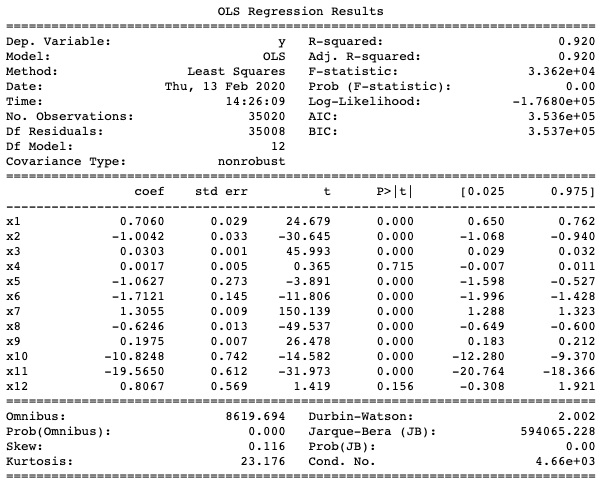
The R-squared value is already much better at 0.920. This time we also obtain a much better RMSE:

y_pred = results.predict(np.asarray(X_test))

mse = mean_squared_error(np.asarray(y_test), y_pred)
rmse = mse**0.5
print(rmse)

39.51583952089907

The effect of our attempt at feature engineering is quite drastic since it cut our RMSE in half. We can also implement models other than Ordinary Least Squares (OLS) model. In fact, the statsmodels package has a host of other regression models we can try. The syntax is almost identical to the OLS implementation, so feel free to try a few others to see if a better RMSE is possible (spoiler: OLS seems to be one of the better models, even if it is the simplest).

There is, however, a more advanced model that can produce a slightly better result. For this, we need the xgboost package. Extreme gradient boosting is an algorithm that involves building multiple weak predictive models, and iteratively minimizing a cost function (or in our case, the RMSE) that results in a single strong predictive model. For a more in-depth discussion on the xgboost algorithm.

To apply the xgboost algorithm in Python:

import xgboost as xgb

dtest = xgb.DMatrix(X_test, y_test, feature_names=X_test.columns)
dtrain = xgb.DMatrix(X_train, y_train,feature_names=X_train.columns)

param = {'verbosity':1,
        'objective':'reg:squarederror',
        'booster':'gblinear',
        'eval_metric' :'rmse',
        'learning_rate': 1}

evallist = [(dtrain, 'train')]

Now iterate:

num_round = 20
bst = xgb.train(param, dtrain, num_round, evallist)

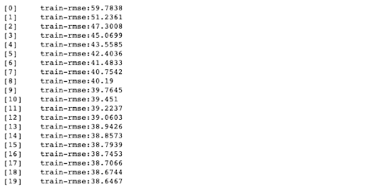
Using the xgboost algorithm, we obtain a slightly better RMSE (~38.6 compared to ~39.5). Feel free to try different learning rates or number of iterations to see how the result changes.

Summary

This post is a demonstration of how to build a prediction model to predict future events. In this project, it predicts the concentration of PM2.5 pollutants in the air in Beijing based on the local weather. With This demonstration, you should be confident to get your hand on the project. before you do, please aware of:

• Using a dataset’s features “as-is” can result in a poorly performing predictive model.
• Feature engineering can play a large role in determining the efficacy of a predictive model.
• Sometimes the simplest statistical model can outperform more sophisticated ones.

In practical terms, applying predictive models to real world problems can help find non-obvious correlations, or confirm suspected ones. And if reliable predictive results can be found, they remove (or at least decrease) the need for real world infrastructure that have significant costs associated with them.

However what is hard and expected from you are:

• explain your model’s performance in a credit way
• efforts you spend to improve it (possibly with other models)
• the detailed evaluation of the model you finally produced

References

• Sample code.
• dataset.
• Tutorial blog

Follow @GaryLi

Last updated: 27/03/2020